Image Hash Roadmap

1 问题引出

1.1 从最近邻搜索谈起(nearest neighbor search, NN)

最近邻检索：给定一张查询图片q(即query)（或文本），从数据库\(\mathcal{X}\)中找到与之最相近的N张图片（或文本）。在实际的检索场景中，我们会用一条向量来作为图片(或文本)的表征。

用公式表达最近邻检索： \[ \mathrm{NN}(q)=\mathrm{arg}\mathop{min}\limits_{x\in \mathcal{X} } \ \mathrm{dist}(q, x) \] dist 是某一种距离计算公式（如欧式距离、余弦距离）

直觉来看，最近邻问题很简单，只要计算query和库中所有向量的距离，再按照距离的大小排序返回最相近样本的索引即可。但是当数据规模过大时这就成为了一个问题。假设查询图片的向量维度为256（即\(d\in \mathbb{R}^{256}\)）,数据了类型为float64，一条向量的数据大小为 256 * 64 / 8 = 2KB。此时采用这种暴力搜索的方法进行检索，代价会非常大。

（实验CPU：Intel(R) Xeon(R) Gold 6226R CPU @ 2.90GHz）

数据库规模	距离计算耗时	向量数据库大小
一百万	\(\sim\) 24.13s秒	\(\sim\) 2GB
一千万	\(\sim\) 4分钟	\(\sim\) 20GB
一亿	\(\sim\) 40分钟	\(\sim\) 200GB

可见当数据量较大时，无论是从向量存储还是从搜索时延都无法满足实际应用需求。在工程中，当向量维度较低时，我们常用Kd-tree来加速搜索。当数据规模过大是（亿级），我们往往用到近似最近邻搜索技术(approximate nearest neighbor search，ANN)，ANN技术的核心技术之一就是向量量化技术(vector quantization, VQ¹)，常用的方法有乘积量化（product quantization，PQ²）,哈希等。

1.2 图片向量哈希是啥，有啥难点

1.2.1 图片向量哈希是啥

向量哈希是ANN技术中向量量化技术的一种常用方法。其目标是学习一个哈希量化函数将一个浮点型或整型的向量量化为一个哈希向量（仅含有两个值，0/1或-1/1）且尽可能的保证搜索结果能够维持（即 similarity preserving）。此时公式（1）可转化为： \[ \mathrm{HashNN}(q)=\mathrm{arg}\mathop{min}\limits_{x\in \mathcal{X} } \ \mathrm{HammingDist}(q, x) \]

\[ \mathrm{HammingDist}(x_1, x_2)=\mathrm{sum}( x1 \oplus x2) \]

通过上面可以看出图片哈希检索与经典的NN检索有两个主要的不同点：

图片向量数据类型不同。哈希向量数域集合只有两个值{-1, 1}，浮点向量的数域集合接近无穷。这个特性能够大大降低向量检索任务的内存消耗。以上文256位的向量为例，数据类型为float64时一条向量占用2KB。但为哈希向量时一条数据类型仅为 256 * 1 / 8 = 32B,降低64倍的存储空间。可见哈希能够大幅度降低磁盘、内存的消耗。

数据库规模 float64向量数据库大小哈希向量数据库大小

一百万 \(\sim\) 2GB \(\sim\) 31 MB

一千万 \(\sim\) 20GB \(\sim\) 310 MB

一亿 \(\sim\) 200GB \(\sim\) 3GB
距离计算公式不同。哈希检索用hamming距离作为其距离计算指标。即对两个向量按位求异或后相加。相对浮点数欧式距离、余弦距离的计算更快。

数据库规模	float64向量数据库大小	哈希向量数据库大小
一百万	\(\sim\) 2GB	\(\sim\) 31 MB
一千万	\(\sim\) 20GB	\(\sim\) 310 MB
一亿	\(\sim\) 200GB	\(\sim\) 3GB

1.2.2 图片向量哈希的主要难点（要解决什么问题）

难点1: 如何解决相似度维持问题（similarity preserving）。即如何保证哈希后的检索结果和原向量的检索结果尽可能的一致。 \[ \mathrm{NN}(q) \simeq \mathrm{HashNN}(q) \] 难点2: 向量哈希需要将向量从浮点数（或整数）映射到只包含两个值的数域空间（0/1或-1/1），这往往会用到符号函数。但符号函数不可导，如何用梯度下降进行优化？（针对用深度学习的哈希方法）。

2 图片向量哈希方法

2.1 相似度维持的解决方案

在深度哈希任务中，主要通过设计特定的损失函数来解决相似度维持问题。

2.1.1 基于成对标签

比较有代表性的是DSH³,DSDH⁴,DPSH⁵等。假定网络输入的图片\(x_1, x_2\),经过网络输出的浮点向量为\(f_1, f_2\)，经过哈希层后得到的哈希向量分别为\(b_1, b_2, b_i \in \{-1, 1\}^c\)，c是哈希向量的维度。成对标签规则如下：

若\(x_1, x_2\)归属同一个类别（或认为相似），则认为其成对标签\(s_{12}=1\)
若\(x_1, x_2\)归属同不同类别否则为\(s_{12}=0\)。

对于任意两个数据点\(i,j\)其似然概率定义如下

\[ p(s_{ij} | \mathcal{B}) = \left \{ \begin{aligned} & \sigma(\Omega_{ij}) \, & s_{ij} = 1 \\ & 1 - \sigma(\Omega_{ij}) \, & s_{ij} = 0 \end{aligned} \right. \] 其中 \(\Omega_{ij}=\frac{1}{2}b_i^Tb_j\)，\(\sigma(\Omega_{ij})=\frac{1}{1+e^{-\Omega_{ij} } }\)

其目标函数为 \[ \mathop{min}\limits_{\mathcal{B} }=- \mathop{log} p(\mathcal{S}|\mathcal{B})=-\sum \limits_{s_{ij} \in \mathcal{S} } \mathop{log} p(s_{ij}| \mathcal{B})=-\sum \limits_{s_{ij} \in \mathcal{S} } (s_{ij} \Omega_{ij} - log(1 + e^{\Omega_{ij} })) \] 此类方法的扩展有：引入margin来优化类内方差与类间方差⁶、扩展到三元组⁷、基于类别分布进行加权⁸、亦或是扩展到多标签⁹

2.1.2 基于语义标签

这类方法很多时候和成对标签损失一起用¹⁰。主要思想是：当我们有图片的标签时，只考虑pairwise信息没有充分利用到标签信息，故增加一个分类的损失来协助训练。 \[ \sum_{i=1}^{N}L(y_i, W^Tb_i) \] 主流的分类损失有3种：1）交叉熵损失；2）浮点向量投影得到的概率向量与哈希向量投影得到的二值向量的KL散度；3）L2损失。

2.1.3 基于相似度一致

假定\(f\)输入图片的浮点特征向量，\(b\)是输入图片的哈希向量。对于一个batch的浮点向量为\([f_1, f_2, ..,, f_N]\)，哈希向量为\([b_1, b_2, ..., b_N]\)浮点向量构成的相似度矩阵\(S_f=[[f_1f_1^T, f_1f_2^T, ..., f_1f_N^T]; ...; [f_Nf_1^T, f_Nf_2^T, ..., f_Nf_N^T]]\)。哈希向量构成的相似度矩阵\(S_b=[[b_1b_1^T, b_1b_2^T, ..., b_1b_N^T]; ...; [b_Nb_1^T, b_Nb_2^T, ..., b_Nb_N^T]]\)

在实际的应用中有直接用MSE来使相似度矩阵最小化；也有利用对比学习思想构造相似度矩阵用交叉语义一致性来优化¹¹。也有直接利用Batch本身标签的相似度矩阵\(S\)来和哈希形成相似度矩阵\(S_b\)进行优化¹²。

2.1.4 基于重建

此类方法一般基于VAE架构。其核心思想是：将浮点向量进行哈希量化后，再用哈希向量进行重建，优化目标是重建后与重建前的feature map尽可能的接近。

比较有代表性的工作是TBH¹³，相较基础的VAE架构同时引入了图卷积来进一步同步哈希向量和浮点向量的特征。

2.1.5 其它相似度维持损失函数

如优化检索排序的 SortedNCE¹⁴，优化哈希码聚类分布的 CSQ¹⁵，基于优化对比量化损失的MeCoQ¹⁶等。

2.1.6 优化哈希码一些约束

为了避免过拟合往往会增加一个量化损失，使得生成的哈希向量与原向量量化误差别太大。一版采用L2损失或SmoothL1。 \[ L_{quan} = \sum_i ^ N{ \parallel b_i - f_i \parallel ^2 } \] 为了使得生成的哈希向量差异性更大往往会增加一个平衡损失使得生成的哈希向量1/-1的个数差不多。 \[ L_{balance}=\frac{1}{N} \parallel BB^T - I \parallel ^2 \]

2.2 符号函数不可导的解决方案

2.2.1 改写梯度更新规则

Pytorch提供了自定义梯度更新的接口。有代表性的GreedyHash¹⁷所用的方法前向过程调用符号函数，反向过程不计算符号函数的梯度。实现的关键是Pytorch中的torch.autograd.Function

class GreedyHashLayer(torch.autograd.Function):
 
    @staticmethod
    def forward(ctx, input):
        return input.sign()
 
    @staticmethod
    def backward(ctx, grad_output):
        return grad_output

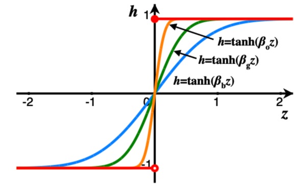
2.2.2 基于“松弛”（relaxation）思想训练中替代符号函数为其它可导函数

此类方法是image hash最为常用的方法。核心思想是：在训练过程将二值化函数用一个可微的函数替代，在推理过程中再用符号函数进行二值化。

3 构建专利图片哈希检索系统

3.1 问题分析及技术选型

目前线上已刷1亿+外观向量，1亿+实用新型向量，4亿+发明专利向量。现阶段我们所用image2vector的pipeline为 图像 -> 去白边 -> （提轮廓, shape-only）-> resize -> 特征提取 -> PCA降维。若采用全量训练的方式更新image2vector模型需要全量重刷已有的向量，代价很大。并且目前自训的模型还达不到Facebook在数十亿规模数据训练的基础模型。

本实验采用的image2hash架构为：固定特征提取模块，在已有pipeline上增加一个哈希层达到image2hash的效果。通过对论文的调研，可以尝试的方向有两大类，一类基于模型，一类基于统计。

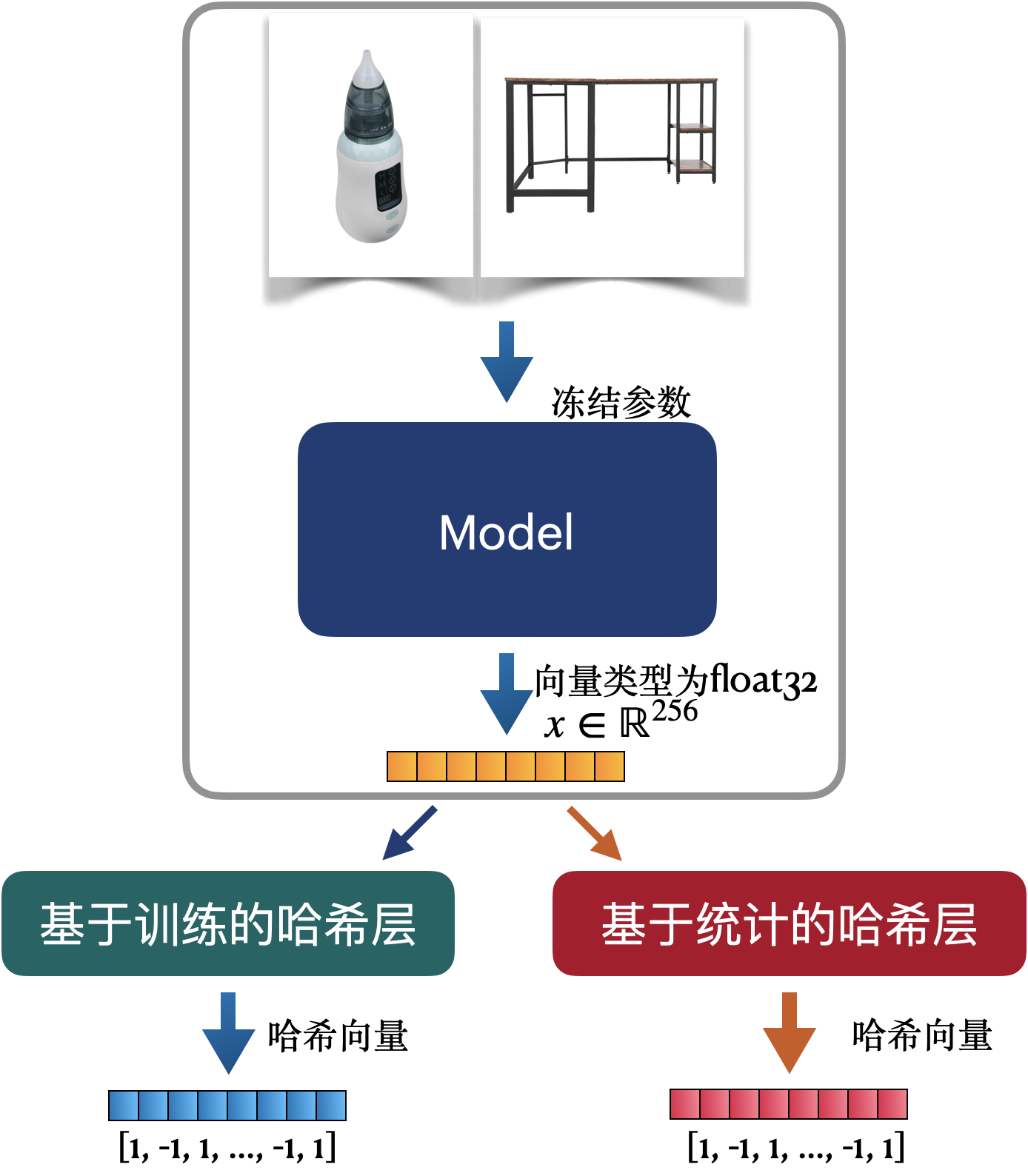
3.1.1 采用模型训练向量哈希参数

与论文场景不同，此处需要将特征提取模块（backbone）的权重全部冻结，只训练哈希层的权重。主要有三类可行的方法：

1）可用公开数据结合标签语义损失+量化损失+平衡损失等进行训练。

2）用专利数据采用自监督的方法进行训练。

3）亦或者直接用最小化浮点向量和哈希向量的量化误差进行训练。

3.1.1.1基于开源数据训练哈希参数

为了快速验证模型效果，首先在imagenet100上进行验证。复现了几个主流的基于深度学习训练哈希层的方法，并在imagenet100上进行测试。（Dbhash是参考Dbnet思想构建的方法）。从结果上，当模型收敛，几类方法的mAP差距不大，但Dbhash的收敛速度特别快，故采用Dbhash架构来训练哈希层。

epoch	Dbhash	GreedyHash¹⁸	CSQ¹⁹	DHN²⁰	DPSH²¹
10	88.61%	86.82%	68.88%	65.85%	66.18%
20	90.27%	89.46%	78.02%	74.81%	75.88%
30	90.34%	90.00%	82.14%	81.87%	82.50%
40	90.48%	90.21%	84.64%	85.72%	86.03%
50	90.55%	90.27%	85.94%	88.11%	88.09%
60	90.53%	90.56%	86.86%	89.58%	89.28%
70	90.60%	90.60%	87.57%	90.75%	89.89%
80	90.59%	90.59%	88.20%	91.56%	90.37%

DBhash 模型架构

整体架构如下图所示，需要训练的哈希层为Thresh layer。

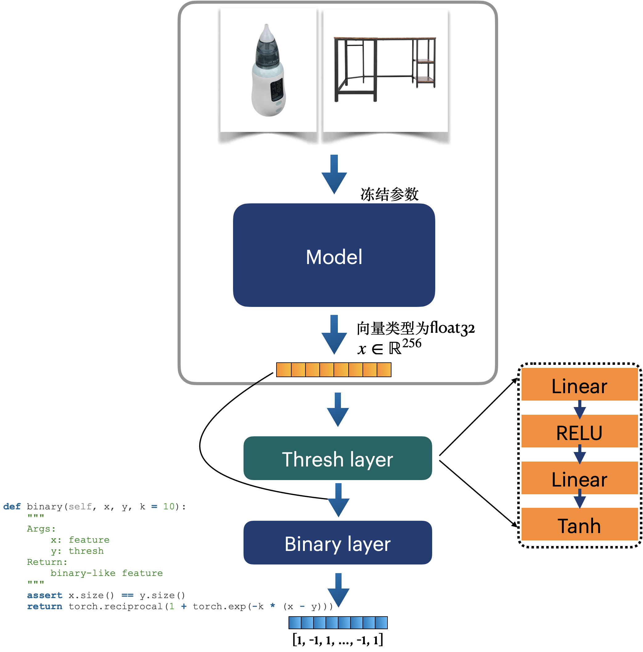
训练目标函数有3个：语义标签分类损失、KL散度及量化损失。（效果见3.3.1）

训练数据：imagenet1K

PS：在实际尝试的过程中发现一个坑。BN层的统计数据(running_mean, running_var)更新是在每一次训练阶段model.train()后的forward()方法中自动实现的，而不是在梯度计算与反向传播中更新optim.step()中完成。采用require_grad=False这个方法无法正常冻结。正确的冻结BN的方式是在模型训练时，把BN单独挑出来，重新设置其状态为eval (在model.train()之后覆盖training状态）

def set_bn_eval(m):
    classname = m.__class__.__name__
    if classname.find('BatchNorm') != -1:
      m.eval()

model.apply(set_bn_eval)

3.1.1.2直接基于最小化量化误差来训练哈希层

本次POC主要尝试了iteration quantization（ITQ²²）。这个方法的核心思路是将经过PCA的向量数据集中的数据点映射到一个二进制超立方体的顶点上，使得对应的量化误差最小，从而而已得到对应该数据集优良的二进制编码。其核心思路是：找到最优的旋转投影矩阵来使得量化误差最小。代码实现如下：

class ITQ:
    """training hash code by ITQ method"""
    DEFAULT_DEVICE = torch.device("cuda") if torch.cuda.is_available() else torch.device("cpu")
    def __init__(self, device=DEFAULT_DEVICE):
        self.device = device

    def __call__(self):
        pass 
    
    def train_pipeline(
            self, 
            vec_rtpath, 
            file_type, 
            pca_file=None, 
            checkpoints=None, 
            iterations=1000, 
            thred=None, 
            debug=False
            ) -> None:
        trainset = self.prepare_patent_data(
            vec_rtpath, file_type, pca_file=pca_file, debug=debug
        )
        self.train(
            trainset, checkpoints=checkpoints, iterations=iterations, thred=thred
        )

    def prepare_patent_data(self, vec_rtpath, file_type, pca_file=None, debug=False):
        vector_ls, image_ls = VectorFileDecoder(file_type=file_type)(
            vec_rtpath, sample_number=30 if debug else -1
        )
        if pca_file is None:
            pca_func = lambda x: x 
        else:
            pca_func = PCA(pca_file)
        vector_ls = [pca_func(np.array(i).reshape(1, -1)).reshape(-1).tolist() for i in tqdm(vector_ls)]
        vector_arr = np.array(vector_ls)  # N * M
        return vector_arr

    def train(self, trainset: np.ndarray, checkpoints=None, iterations=1000, thred=None):
        trainset_tensor = torch.from_numpy(trainset.astype(np.float32)).to(self.device)
        V = trainset_tensor
        nbits = trainset_tensor.shape[1]
        R = torch.randn(nbits, nbits).to(self.device) 
        torch.nn.init.orthogonal_(R)
        origin_quan_loss = self.frobenius_norm(V.sign(), V)
        if thred is not None:
            binary_vec = FaissSearchAPI.img2hash_by_thred(
                trainset, thred, to_int8_compress=False
            ).astype(np.float32)
            logger.info(f"generate binary vector by OT method: binary vec shape: {binary_vec.shape}")
            origin_quan_loss_2 = self.frobenius_norm(torch.from_numpy(binary_vec).to(self.device), V)
        else:
            origin_quan_loss_2 = 0.0000

        best_quant_loss = 1e10
        best_R = None

        for i in range(iterations):
            # step 1: update B
            V_tilde = V @ R 
            B = V_tilde.sign()
            # step2: update R 
            [S, _, S_tilde_transpose] = torch.svd(B.t() @ V)
            R = (S_tilde_transpose.t() @ S.t())

            quant_loss = self.frobenius_norm(B, V_tilde)
            if quant_loss < best_quant_loss:
                best_quant_loss = quant_loss
                best_R = R 
            logger.info(f"Iter: {i:04d} frobenius_norm: {quant_loss:.4f}, BEST: {best_quant_loss:.4f}, ORIGIN: {origin_quan_loss:.4f}, ORI2: {origin_quan_loss_2:.4f}")
        
        if checkpoints:
            np.savez(checkpoints, R=best_R.cpu().numpy()) 
             

    @staticmethod
    def frobenius_norm(B, V_tilde) -> float:
        """$E = || B - V_tilde ||_{F}^{2}$"""
        return (B - V_tilde).pow(2).sum().sqrt().item() / B.shape[0]

3.1.2 基于统计特征获得向量哈希参数

该方法的本质是挖掘浮点向量的数值分布统计特征，以最小化量化损失、平衡损失为目标来构建哈希层。基于最优传输理论（Op timal Transport, OT）的Bi-HalfNet²³。论文为什么写了很多，感兴趣可以看原文，这里主要讲怎么做。目前我们有1800w的专利图片向量，其构成的矩阵记为\(\mathrm{M}=\{m_i |i=1,2,...,18000000 \}, m_i \in \mathbb{R}^{256}\),对于向量检索任务，向量\(m_i\)可以看作是对应图片\(x_i\)的表征。已知\(m_i\)是256维，基于OT理论的哈希方法是将\(m_i\)的每一维都当作一个特征。已知\(m_i=[m_{i,1}, m_{i,2},...,m_{i,256}]\)。将所有样本第一维的特征汇聚一起可得：\(f_1=\{m_{i1}|i=1,2, ..., 18000000 \}\)，如何得到一个划分，将\(f_i\)转为二值化，且量化误差最小是我们的目标函数，即 \[ \mathop{min} \sum \limits_{j} \parallel f_i^{j} - b_i^{j} \parallel ^ 2 \] \(f_i^{j}\)表示在\(f_i\)的第\(j\)个样本；\(b_i^{j}\)表示\(f_i^{j}\)的哈希表示。

显然\(\mathop{mean} (f_i)\)是我们所需的解。但仅仅考虑量化误差没有兼顾哈希特征的丰富性，在实践中往往会加入一个平衡误差来使得一条哈希向量两个值的数量尽可能的接近。\(f_i\)的中位数是我们所需的解。

综上所述，我们只需分别找到每一维的中位数作为该位置的划分，即可获得最小量化误差、最优平衡的哈希表征。

3.2检索系统搭建

Milvus 1.x并不支持哈希检索。本次POC采用Faiss平台搭建基于哈希的检索系统。（吐槽一下，faiss关于搭建哈希搜索的文档真的非常简略）里面有个大坑是插入哈希code导Faiss引擎是需要将哈希吗转为int8后在输入，随后需要将向量的维度变为 \(\mathrm{dim} /8\)

def bytes2int8(byte_vec):
    """
    convert 0,1 matrix to uint8
    shape: (N, M) -> (N, M // 8)
    """
    assert byte_vec.ndim == 2
    mutiple = np.array([2**i for i in range(7, -1, -1)]).reshape(1, -1)
    hash_code = byte_vec
    hash_code_uint8 = np.concatenate(
        [np.sum(hash_code[:, i * 8 : (i + 1) * 8] * mutiple, axis=1, keepdims=True)
            for i in range(hash_code.shape[1] // 8)],
        axis=1
    ).astype(np.uint8)
    return hash_code_uint8

3.2.1索引构建

class FaissSearchEngin:
    SUPPORT_INDEX_TYPE = set(
        [
            "binary_flat_ivf",
            "binary_flat",
        ]
    )

    def __init__(
        self,
        index_type,
        index_params=dict(),
        index_rtpath=DEFAULT_INDEX_RTPATH,
        vector=None,
        img_name_ls=None, 
        reuse=True,
        logger=logger,
        prefix = '', 
    ) -> None:
        """
        Args:
            index_type(str): faiss index type
            index_params(dict): faiss index create parameters
            index_rtpath(str): faiss index rtpath
            vector(np.ndarray, None): faiss index database
            reuse(bool): always create index, whatever
        """
        self.logger = logger
        self.reuse = reuse
        self.index_type =  index_type
        assert (
            index_type in self.SUPPORT_INDEX_TYPE
        ), f"index type only support {self.SUPPORT_INDEX_TYPE} now!"
        self.vector = vector
        self.img_name_ls = img_name_ls
        if self.vector is not None:
            dim = vector.shape[1] * 8 if "binary" in self.index_type else vector.shape[1]
            index_params.update(dict(dim=dim))
        self.logger.info(f"index params: {index_params}")
        self.index_save_rtpath = os.path.join(index_rtpath, index_type)
        self.index_path = os.path.join(
            self.index_save_rtpath,
            f"{prefix}_{'_'.join([f'{k}_{v}' for k, v in index_params.items()])}.index",
        )
        self.index_params = index_params
        checkdir(self.index_save_rtpath)

    def run(self):
        self.check_index()
        self.init_index_func(self.index_type)
        self.index = self.build_index(
            self.vector, index_params=self.index_params, index_path=self.index_path, reuse=self.reuse
        )

    def check_index(self):
        if self.reuse and self.vector is None:
            assert os.path.exists(
                self.index_path
            ), f"there are no index file, you should input [vector] parameters to create it"

    def convert_byte_vector_2_uint8(self):
        pass 

    def init_index_func(self, index_type):
        if index_type == "binary_flat_ivf":
            self._index_func = self._binary_flat_ivf
            self.write_index_func = faiss.write_index_binary
            self.read_index_func = faiss.read_index_binary
        elif index_type == "binary_flat":
            self._index_func = self._binary_flat
            self.write_index_func = faiss.write_index_binary
            self.read_index_func = faiss.read_index_binary
        else:
            raise NotImplementedError

    def search(self, query, search_params):
        D, I = self.index.search(query, **search_params)
        return D, I

    def build_index(self, vector, index_path, index_params=dict(), reuse=False):
        """create faiss index"""
        if os.path.exists(index_path) and reuse:
            self.logger.info(f"read index from exists file: {index_path}")
            return self.read_index_func(index_path)
        else:
            index_info = self._index_func(index_params)
            vector = vector.astype(index_info.vec_dtype)
            self.logger.info(f"vector shape: {vector.shape}, dtype: {vector.dtype}")
            if index_info.need_train:
                self.logger.info(f"start train index, please wait...")
                _t = time.perf_counter()
                index_info.index_func.train(vector)
                self.logger.info(
                    f"train index finish, time consume: {time.perf_counter() - _t}s"
                )
            else:
                self.logger.info(f"current index type need not to train!")
            index_info.index_func.add(vector)
            self.save_id_map(self.index_path.replace(".index", "_id_map.txt"))
            self.logger.info(f"save index file to {index_path}")
            self.write_index_func(index_info.index_func, index_path)
            return index_info.index_func

    def _binary_flat(self, params):
        index = faiss.IndexBinaryFlat(params.get("dim"))
        return index_info(index, False, np.uint8)

    def _binary_flat_ivf(self, params):
        quantizer = faiss.IndexBinaryFlat(params.get("dim"))
        index = faiss.IndexBinaryIVF(quantizer, params.get("dim"), params.get("nlist"))
        return index_info(index, True, np.uint8)

    def train(self, index, training_vector):
        self.logger.info(f"start train index")
        _t = time.perf_counter()
        index.train(training_vector)
        self.logger.info(f"train index succeed! time consume: {time.perf_counter() - _t:.4f}s")
        assert index.is_trained, f"index not train!"
    
    def save_id_map(self, save_path):
        checkdir(os.path.split(save_path)[0])
        with open(save_path, 'w', encoding="utf-8") as f:
            f.write('\n'.join(self.img_name_ls))

3.3 指标及web demo搭建

3.3.1 指标评估

分别在灰度测试集和轮廓测试集来测试哈希检索的效果。baseline为SQ8量化（目前线上的量化方式）

候选数据集：140W 外观专利图片数据

测试集：外观专利灰度测试集、外观专利轮廓测试集

3.3.1.1 精度评估

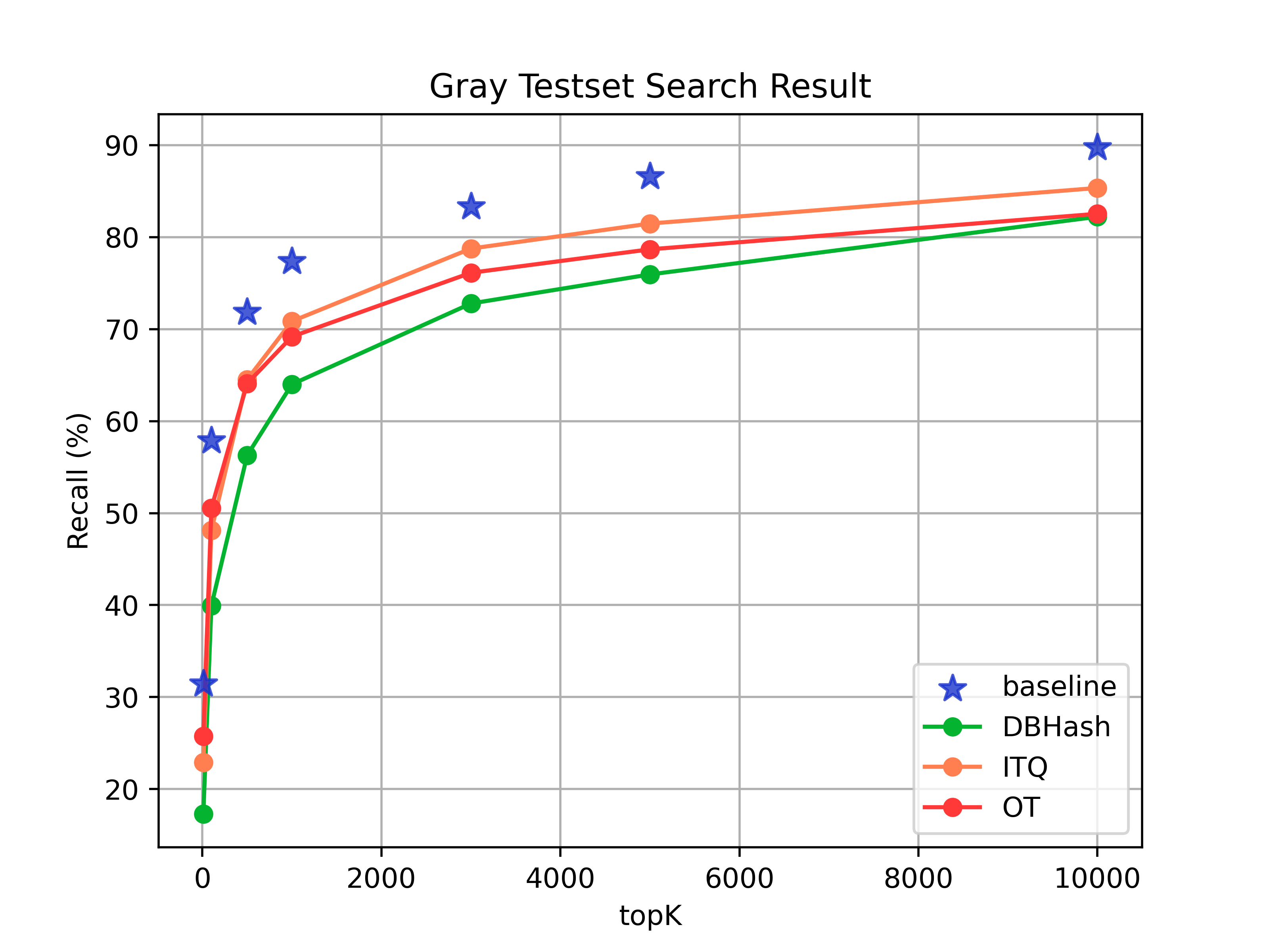
灰度测试集的效果对比

topk	baseline	哈希检索（Dbhash）	哈希检索（ITQ）	哈希检索(OT)
10	31.43%	17.30%	22.91%	25.73%
100	57.86%	39.95%	48.11%	50.54%
500	71.82%	56.28%	64.53%	64.09%
1000	77.35%	64.00%	70.85%	69.18%
3000	83.32%	72.78%	78.75%	76.12%
5000	86.57%	75.94%	81.47%	78.67%
10000	89.73%	81.21%	85.34%	82.53%

轮廓测试集的效果对比

topk	baseline	哈希检索（Dbhash）	哈希检索（ITQ）	哈希检索(OT)
10	4.97%	4.67%	4.19%	5.51%
100	12.21%	12.33%	9.16%	14.00%
500	21.48%	22.20%	15.74%	26.03%
1000	27.53%	28.61%	20.59%	33.21%
3000	37.64%	38.78%	29.44%	42.85%
5000	41.17%	43.57%	33.45%	46.92%
10000	46.62%	52.00%	38.90%	52.24%

从实验结果看，采用OT方法进行哈希量化能达到最优的效果。并且该方法实现简单，能够复用已刷的向量。

3.3.3.2 向量存储评估

以目前256维向量为例。线上采用SQ8量化相较float32存储占用少4倍。哈希量化存储量化在SQ8基础上还能少8倍。

3.3.1.3 检索速度评估

候选集大小：140W

测试数据量： 100条

检索类型	平均检索耗时
SQ8检索	50.11m s
哈希检索	24.92ms

哈希检索较SQ8速度提升50.31%

3.3.2 web demo

检索类型	web demo 地址
常规的SQ8搜索	http://192.168.18.240:20002/baseline
哈希搜索	http://192.168.18.240:20002/binary_flat_ivf

3.4 结论

本次POC调研了image hash的常用算法，并在专利图片检索中进行尝试。并对哈希搜索的精度、速度有了一定的认知。

精度上：

灰度测试集在top1k召回上，哈希搜索较向量搜索降低8.17% （77.35% -> 69.18%）。但是哈希检索top3K的召回能达到76.12%。若后续做重排的话，粗筛可用哈希搜索。
轮廓测试集在top1k召回上，哈希搜索较向量搜索提升4.68% (27.53% -> 33.21%)

存储上：

哈希向量比原浮点型内存占用降低32倍，较SQ8向量内存占用降低8倍。

检索速度上：

哈希搜索相较SQ8提升50.13%（gallery 140w）

后续可以应用的方向目前来看有2个：

对于粗精排检索范式，可在粗排阶段用哈希做召回，精排阶段用浮点向量做排序。
精度要求不高的检索场景可用哈希检索。

4 附录：图片哈希检索的经典论文

4.1 图片哈希检索经典论文

Model	Learning Paradiam	Loss Function	Benchmark	Publish	Cite	year
CNNH²⁴	有监督			AAAI	949	2014
SDH²⁵	有监督	标签语义损失，量化损失	CIFAR-10,NUS-WIDE,MNIST,ImageNet100	CVPR	1121	2015
DSH²⁶	有监督	成对标签损失，量化损失	CIFAR-10,NUS-WIDE	CVPR	774	2016
DPSH²⁷	有监督	成对标签损失，量化损失	CIFAR-10,NUS-WIDE	IJCAI	607	2016
DTSH²⁸	有监督	三元组对损失，量化损失	CIFAR-10,NUS-WIDE	-	168	2016
DHN²⁹	有监督	成对标签损失，量化损失	CIFAR-10,NUS-WIDE,Flickr	AAAI	563	2016
HashNet³⁰	有监督	加权成对标签损失，量化损失	ImageNet100,NUS-WIDE,MS COCO	ICCV	503	2017
DSDH³¹	有监督	成对标签损失，语义标签损失，量化损失	CIFAR-10,NUS-WIDE	NIPS	243	2017
LCDSH³²	有监督	成对标签损失，量化损失	CIFAR-10,NUS-WIDE	IJCAI	13	2017
DAPH³³	有监督	成对标签损失，平衡损失，量化损失	CIFAR-10,NUS-WIDE	ACM	105	2017
GreedyHash³⁴	有监督	语义标签损失，量化损失	CIFAR-10,ImageNet100	NIPS	100	2018
DCH³⁵	有监督		CIFAR-10,NUS-WIDE,MS COCO	CVPR	258	2018
DFH³⁶	有监督	带margin的成对标签损失，语义标签损失，量化损失	CIFAR-10,ImageNet100	BMVC	15	2019
IDHN³⁷	有监督，多标签	成对多标签损失，量化损失	NUS-WIDE,Flickr,VOC2012,IAPRTC12	IEEE	82	2019
DAGH³⁸	有监督	成对标签损失，量化损失，平衡损失	CIFAR-10,NUS-WIDE,Fashion-MNIST	ICCV	43	2019
DSHSD³⁹	有监督	成对标签L2损失，语义标签损失	CIFAR-10,NUS-WIDE,ImageNet100	IEEE	11	2019
DistillHash⁴⁰	无监督			CVPR	105	2019
SPDAQ⁴¹	有监督	相似度维持损失，平衡损失，量化损失	CIFAR-10,NUS-WIDE-21,NUS-WIDE-81,MS-COCO	AAAI	12	2019
DBDH⁴²	有监督	成对标签损失，平衡损失	MNIST,CIFAR-10,CIFAR-20,Youtube Faces	-	31	2020
CSQ⁴³	有监督	平衡损失，基于聚类的量化损失	UCF101,HMDB51,ImageNet100, MS COCO,NUS-WIDE	CVPR	133	2020
TBH⁴⁴	无监督	重建损失，差异判别损失	CIFAR-10,NUS-WIDE,MS COCO	CVPR	67	2020
DPAH⁴⁵	有监督，多标签	差异正则损失，类间距离差异损失	NUS-WIDE,MS COCO,ImageNet100	WACV	13	2020
ICICH⁴⁶	有监督，跨模态	-	WIKI,MIRFlickr,NUS-WIDE	-	12	2020
TSDH⁴⁷	有监督	类内中心损失，相似矩阵一致性损失	CIFAR-10,NUS-WIDE,Flickr25K	TNNLS	73	2020
DDDH⁴⁸	有监督	成对标签损失，语义标签损失，量化损失	CIFAR-10,NUS-WIDE,MS COCO	-	8	2020
EDSH⁴⁹	有监督，跨模态	-	WIKI,MIRFlickr25K,NUS-WIDE	-	21	2020
SPLH⁵⁰	有监督	相似度维持损失	CIFAR-10,MINIST,Places205	IEEE	30	2020
Bi-Half Net⁵¹	无监督	量化损失	CIFAR-10,MS COCO,MNIST,UCF101,HMDB51	AAAI	24	2021
CIBHash⁵²	无监督，对比	对比损失	CIFAR-10,NUS-WIDE,MS COCO	-	13	2021
CIMON⁵³	有监督，对比	平行语义一致性损失，交叉语义一致性损失，对比一致损失	CIFAR-10,NUS-WIDE,Flickr25K	-	14	2021
SPQ⁵⁴	有监督，对比	交叉对比损失	CIFAR-10,NUS-WIDE,Flickr25K	ICCV	19	2021
BNNH⁵⁵	有监督	相似度维持损失，激活感知损失	CIFAR-10,MNIST,ImageNet100	-	6	2021
DCDH⁵⁶	有监督	成对标签损失，类间差异似然损失，语义标签回归损失	YouTube Faces,FaceScrub,CFW-60K,VGGFace2	PR	13	2021
DATE⁵⁷	无监督	语义维持损失，对比损失	CIFAR-10,Flickr25K,NUSWIDE-10,NUSWIDE-21	MM	7	2021
SortedNCE⁵⁸	有监督	排序损失	CIFAR-10,NUS-WIDE,MS COCO	-	3	2022
MeCoQ⁵⁹	无监督	对比量化损失	CIFAR-10,NUS-WIDE,Flickr25K	AAAI	7	2022
DSPH⁶⁰	有监督，多模态	-	MIRFlickr,NUS-WIDE,Websearch	-	0	2022
Domino⁶¹	有监督，跨模态	-	CelebA,ImageNet,MIMIC-CXR,EEG	ICLR	27	2022
VTS⁶²	有监督	-	CIFAR-10,NUS-WIDE,MS COCO,ImageNet100	ICME	8	2022
CLIP4hashing⁶³	有监督	相似矩阵一致性损失	MSRVTT,DiDeMo,MSVD	ICMR	1	2022

莫叶何竹